For my final project in Urban Ecologies Methods, I am proposing creating a project that looks at the most recent mayoral election. The inspiration for this project comes from the maps released by the New York Times showcasing which areas voted for Zohran Mamdani. This mayoral election was a highly publicized and potentially consequential affair. Historically, the election of outwardly socialist candidates coincided with turmoil leading up to the election. It is important to contextualize New York City within both this time period and the following years leading up to this.
I am particularly interested in the demographic information of the districts that did and did not vote for Zohran Mamdani. What is their income level? their race? My question is, what is the relationship, if there is any, between the relative wealth of an area and the likelihood of voting for Zohran Mamdani for mayor?
This project will look at these correlations on an income and race level. I will pay particular attention to certain geographies, specifically:
Financial District - This was an area that was surprising to many people as it swung towards Zohran.
The “commie corridor” Park Slope/Flatbush/Crown Heights - this was a projected hotbed for Zohran
Upper Eastside - another anticipated hotbed for Cuomo voters
Staten Island - the only borough where Cuomo beat Zohran
South Bronx - a wildcard that has been gentrifying.
Reading layer `nyed' from data source
  `C:\Users\ijkha\Desktop\methods final\data\nyed_25d\nyed.shp'
  using driver `ESRI Shapefile'
Simple feature collection with 4264 features and 3 fields
Geometry type: MULTIPOLYGON
Dimension:     XY
Bounding box:  xmin: 913175.1 ymin: 120128.4 xmax: 1067383 ymax: 272844.3
Projected CRS: NAD83 / New York Long Island (ftUS)
Code
# -------------------------------# 3. Load Election Data (ED-level from BOE)# -------------------------------files <-list.files("C:/Users/ijkha/Desktop/methods final/data", pattern ="Mayor Citywide ED Level", full.names =TRUE)elections_raw <-map_df(files, read_xlsx) %>%clean_names()# Filter Mamdani rowsmamdani_rows <- elections_raw %>%filter(public_counter %in%c("Zohran Kwame Mamdani (Democratic)","Zohran Kwame Mamdani (Working Families)" ))# Filter Cuomo rowcuomo_rows <- elections_raw %>%filter(public_counter =="Andrew M. Cuomo (Fight and Deliver)")# Pivot to long formatmamdani_long <- mamdani_rows %>%pivot_longer(cols =starts_with("x"),names_to ="ed_col",values_to ="votes" ) %>%mutate(votes =suppressWarnings(as.numeric(votes)),ed =as.integer(str_remove(ed_col, "x")) )cuomo_long <- cuomo_rows %>%pivot_longer(cols =starts_with("x"),names_to ="ed_col",values_to ="votes" ) %>%mutate(votes =suppressWarnings(as.numeric(votes)),ed =as.integer(str_remove(ed_col, "x")) )# Aggregate ED votesmamdani_agg <- mamdani_long %>%group_by(ed) %>%summarize(mamdani_votes =sum(votes, na.rm =TRUE))cuomo_agg <- cuomo_long %>%group_by(ed) %>%summarize(cuomo_votes =sum(votes, na.rm =TRUE))votes <-full_join(mamdani_agg, cuomo_agg, by ="ed")# Join to ED geometries + compute winnered_results_geo <- ed %>%left_join(votes, by =c("ed_num"="ed")) %>%mutate(winner =case_when( mamdani_votes > cuomo_votes ~"Mamdani", mamdani_votes < cuomo_votes ~"Cuomo",TRUE~"Tie" ) )# -------------------------------# 4. Download ACS Tract-Level Median Income# -------------------------------income_tracts <-get_acs(geography ="tract",variables ="B19013_001",state ="NY",county =c("New York", "Kings", "Queens", "Bronx", "Richmond"),year =2022,geometry =TRUE) %>%st_transform(st_crs(ed)) %>%rename(median_income = estimate)# -------------------------------# 5. Spatially Assign Tracts → ED# -------------------------------# Intersect tract polygons with ED polygonstract_ed_intersection <-st_intersection( income_tracts %>%select(GEOID, median_income), ed %>%select(ed_num))tract_ed_intersection <- tract_ed_intersection %>%mutate(area =st_area(.))# Assign each tract to the ED containing the largest sharetract_ed_assignment <- tract_ed_intersection %>%group_by(GEOID) %>%slice_max(area, n =1) %>%ungroup() %>%st_drop_geometry() %>%select(GEOID, ed_num, median_income)# -------------------------------# 6. Aggregate Income to ED# -------------------------------ed_income <- tract_ed_assignment %>%group_by(ed_num) %>%summarize(median_income =median(median_income, na.rm =TRUE) )# Combine with voting dataed_results_income <- ed_results_geo %>%left_join(ed_income, by ="ed_num")spearman_df <- ed_results_income %>%st_drop_geometry() %>%select(median_income, mamdani_votes, cuomo_votes) %>%mutate(total_votes = mamdani_votes + cuomo_votes) %>%filter(!is.na(median_income),!is.na(mamdani_votes), total_votes >0 )# Run Spearman correlationspearman_test <-cor.test( spearman_df$median_income, spearman_df$mamdani_votes,method ="spearman")# Extract stats for annotationrho_val <-round(spearman_test$estimate, 3)p_val <-signif(spearman_test$p.value, 3)# Plotspearman_plot <-ggplot( spearman_df,aes(x = median_income, y = mamdani_votes)) +geom_point(alpha =0.4, size =1.5) +geom_smooth(method ="loess",se =TRUE,color ="black",linewidth =0.8 ) +scale_x_continuous(labels = scales::dollar_format()) +scale_y_continuous(labels = scales::comma) +annotate("text",x =Inf,y =Inf,hjust =1.1,vjust =1.5,size =4,label =paste0("Spearman \u03C1 = ", rho_val,"\n p-value = ", p_val ) ) +labs(title ="Median Income vs Mamdani Vote Count (ED Level)",subtitle ="Spearman rank correlation with LOESS smoother",x ="Median Household Income",y ="Mamdani Vote Count",caption ="Source: NYC BOE (ED-level votes) & ACS 2022 5-year estimates" ) +theme_minimal(base_size =12)print(spearman_plot)
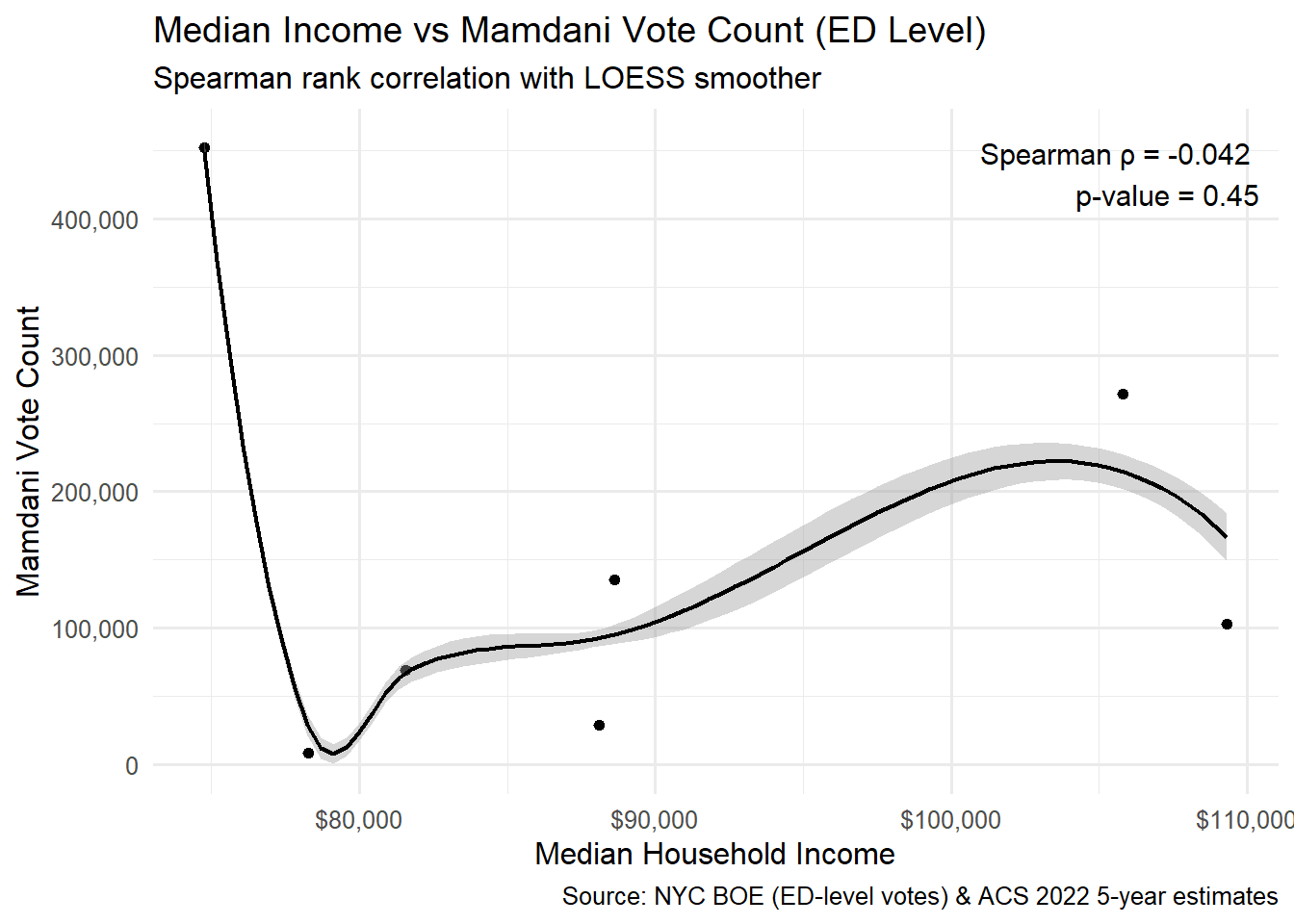
A spearman rank correlation graph showing the relationship between median household income and number of Mamdani votes
Reading layer `nyed' from data source
  `C:\Users\ijkha\Desktop\methods final\data\nyed_25d\nyed.shp'
  using driver `ESRI Shapefile'
Simple feature collection with 4264 features and 3 fields
Geometry type: MULTIPOLYGON
Dimension:     XY
Bounding box:  xmin: 913175.1 ymin: 120128.4 xmax: 1067383 ymax: 272844.3
Projected CRS: NAD83 / New York Long Island (ftUS)
Code
# -------------------------------# 3. Load Election Data (ED-level from BOE)# -------------------------------files <-list.files("C:/Users/ijkha/Desktop/methods final/data",pattern ="Mayor Citywide ED Level",full.names =TRUE)elections_raw <-map_df(files, read_xlsx) %>%clean_names()# Filter Mamdani rowsmamdani_rows <- elections_raw %>%filter(public_counter %in%c("Zohran Kwame Mamdani (Democratic)","Zohran Kwame Mamdani (Working Families)" ))# Filter Cuomo rowcuomo_rows <- elections_raw %>%filter(public_counter =="Andrew M. Cuomo (Fight and Deliver)")# Pivot to long format (candidate votes by ED column)mamdani_long <- mamdani_rows %>%pivot_longer(cols =starts_with("x"),names_to ="ed_col",values_to ="votes" ) %>%mutate(votes =suppressWarnings(as.numeric(votes)),ed =as.integer(str_remove(ed_col, "x")) )cuomo_long <- cuomo_rows %>%pivot_longer(cols =starts_with("x"),names_to ="ed_col",values_to ="votes" ) %>%mutate(votes =suppressWarnings(as.numeric(votes)),ed =as.integer(str_remove(ed_col, "x")) )# Aggregate ED votesmamdani_agg <- mamdani_long %>%group_by(ed) %>%summarize(mamdani_votes =sum(votes, na.rm =TRUE), .groups ="drop")cuomo_agg <- cuomo_long %>%group_by(ed) %>%summarize(cuomo_votes =sum(votes, na.rm =TRUE), .groups ="drop")votes <-full_join(mamdani_agg, cuomo_agg, by ="ed")# Join to ED geometries + compute winnered_results_geo <- ed %>%left_join(votes, by =c("ed_num"="ed")) %>%mutate(winner =case_when( mamdani_votes > cuomo_votes ~"Mamdani", mamdani_votes < cuomo_votes ~"Cuomo",TRUE~"Tie" ) )# -------------------------------# 4. Download ACS Tract-Level Race Counts (B02001)# -------------------------------# Run once if needed (then restart R):# census_api_key("YOUR_KEY", install = TRUE)race_tracts <-get_acs(geography ="tract",variables =c(total ="B02001_001",white ="B02001_002" ),state ="NY",county =c("New York", "Kings", "Queens", "Bronx", "Richmond"),year =2022,geometry =TRUE,output ="wide") %>%st_transform(st_crs(ed)) %>%transmute( GEOID,total = totalE,white = whiteE,nonwhite =pmax(total - white, 0),pct_nonwhite =if_else(total >0, nonwhite / total, NA_real_), geometry )# -------------------------------# 5. Spatially Assign Tracts → ED (largest overlap, like your income script)# -------------------------------tract_ed_intersection <-st_intersection( race_tracts %>%select(GEOID, total, white, nonwhite, pct_nonwhite), ed %>%select(ed_num)) %>%mutate(area =st_area(.))# Assign each tract to the ED containing the largest share of its areatract_ed_assignment <- tract_ed_intersection %>%group_by(GEOID) %>%slice_max(area, n =1, with_ties =FALSE) %>%ungroup() %>%st_drop_geometry() %>%select(GEOID, ed_num, total, white, nonwhite, pct_nonwhite)# -------------------------------# 6. Aggregate Race to ED (population-weighted)# -------------------------------ed_race <- tract_ed_assignment %>%group_by(ed_num) %>%summarize(total_pop =sum(total, na.rm =TRUE),nonwhite_pop =sum(nonwhite, na.rm =TRUE),pct_nonwhite =if_else(total_pop >0, nonwhite_pop / total_pop, NA_real_),.groups ="drop" )# Combine with voting dataed_results_race <- ed_results_geo %>%left_join(ed_race, by ="ed_num")race_winner_map <-ggplot(ed_results_race) +geom_sf(aes(fill = pct_nonwhite), color =NA) +geom_sf(aes(color = winner), fill =NA, size =0.3) +scale_fill_viridis_c(labels =percent_format(accuracy =1), option ="C") +scale_color_manual(values =c("Mamdani"="#b2182b", "Cuomo"="#2166ac", "Tie"="gray60") ) +labs(title ="Race & Voting Patterns at ED Level",subtitle ="Fill = % Non-White (ACS est.); border = winner",color ="Winner",fill ="% Non-White" ) +theme_minimal()print(race_winner_map)
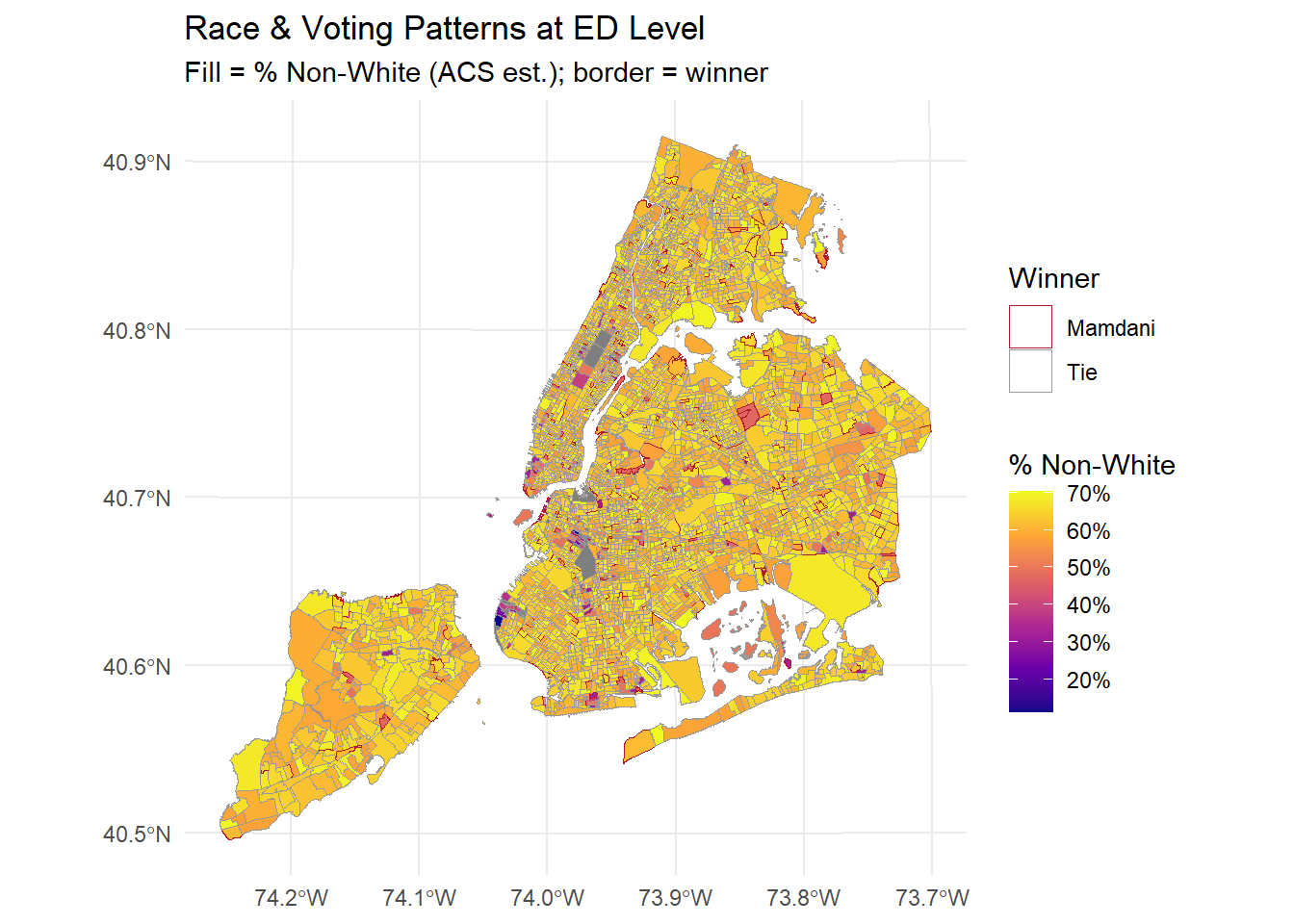
A Choropleth map showing white v.s non-white percentage at ED level with red borders showing EDs that Mamadani won
Reading layer `nyed' from data source
  `C:\Users\ijkha\Desktop\methods final\data\nyed_25d\nyed.shp'
  using driver `ESRI Shapefile'
Simple feature collection with 4264 features and 3 fields
Geometry type: MULTIPOLYGON
Dimension:     XY
Bounding box:  xmin: 913175.1 ymin: 120128.4 xmax: 1067383 ymax: 272844.3
Projected CRS: NAD83 / New York Long Island (ftUS)
Code
# -------------------------------# 3. Load Election Data (ED-level from BOE)# -------------------------------files <-list.files("C:/Users/ijkha/Desktop/methods final/data",pattern ="Mayor Citywide ED Level",full.names =TRUE)elections_raw <-map_df(files, read_xlsx) %>%clean_names()# Filter Mamdani rowsmamdani_rows <- elections_raw %>%filter(public_counter %in%c("Zohran Kwame Mamdani (Democratic)","Zohran Kwame Mamdani (Working Families)" ))# Filter Cuomo rowcuomo_rows <- elections_raw %>%filter(public_counter =="Andrew M. Cuomo (Fight and Deliver)")# Pivot to long format (candidate votes by ED column)mamdani_long <- mamdani_rows %>%pivot_longer(cols =starts_with("x"),names_to ="ed_col",values_to ="votes" ) %>%mutate(votes =suppressWarnings(as.numeric(votes)),ed =as.integer(str_remove(ed_col, "x")) )cuomo_long <- cuomo_rows %>%pivot_longer(cols =starts_with("x"),names_to ="ed_col",values_to ="votes" ) %>%mutate(votes =suppressWarnings(as.numeric(votes)),ed =as.integer(str_remove(ed_col, "x")) )# Aggregate ED votesmamdani_agg <- mamdani_long %>%group_by(ed) %>%summarize(mamdani_votes =sum(votes, na.rm =TRUE), .groups ="drop")cuomo_agg <- cuomo_long %>%group_by(ed) %>%summarize(cuomo_votes =sum(votes, na.rm =TRUE), .groups ="drop")votes <-full_join(mamdani_agg, cuomo_agg, by ="ed")# Join to ED geometries + compute winnered_results_geo <- ed %>%left_join(votes, by =c("ed_num"="ed")) %>%mutate(winner =case_when( mamdani_votes > cuomo_votes ~"Mamdani", mamdani_votes < cuomo_votes ~"Cuomo",TRUE~"Tie" ) )# -------------------------------# 4. Download ACS Tract-Level Race Counts (B02001)# -------------------------------# Run once if needed (then restart R):# census_api_key("YOUR_KEY", install = TRUE)race_tracts <-get_acs(geography ="tract",variables =c(total ="B02001_001",white ="B02001_002" ),state ="NY",county =c("New York", "Kings", "Queens", "Bronx", "Richmond"),year =2022,geometry =TRUE,output ="wide") %>%st_transform(st_crs(ed)) %>%transmute( GEOID,total = totalE,white = whiteE,nonwhite =pmax(total - white, 0),pct_nonwhite =if_else(total >0, nonwhite / total, NA_real_), geometry )# -------------------------------# 5. Spatially Assign Tracts → ED (largest overlap, like your income script)# -------------------------------tract_ed_intersection <-st_intersection( race_tracts %>%select(GEOID, total, white, nonwhite, pct_nonwhite), ed %>%select(ed_num)) %>%mutate(area =st_area(.))# Assign each tract to the ED containing the largest share of its areatract_ed_assignment <- tract_ed_intersection %>%group_by(GEOID) %>%slice_max(area, n =1, with_ties =FALSE) %>%ungroup() %>%st_drop_geometry() %>%select(GEOID, ed_num, total, white, nonwhite, pct_nonwhite)# -------------------------------# 6. Aggregate Race to ED (population-weighted)# -------------------------------ed_race <- tract_ed_assignment %>%group_by(ed_num) %>%summarize(total_pop =sum(total, na.rm =TRUE),nonwhite_pop =sum(nonwhite, na.rm =TRUE),pct_nonwhite =if_else(total_pop >0, nonwhite_pop / total_pop, NA_real_),.groups ="drop" )# Combine with voting dataed_results_race <- ed_results_geo %>%left_join(ed_race, by ="ed_num")# ============================================================# 12. SPEARMAN CORRELATION — RACE vs MAMDANI VOTES# ============================================================# Prepare analysis dataframespearman_race_df <- ed_results_race %>%st_drop_geometry() %>%select(pct_nonwhite, mamdani_votes, cuomo_votes) %>%mutate(total_votes = mamdani_votes + cuomo_votes) %>%filter(!is.na(pct_nonwhite),!is.na(mamdani_votes), total_votes >0 )# Run Spearman correlation (asymptotic p-value due to ties)spearman_race_test <-cor.test( spearman_race_df$pct_nonwhite, spearman_race_df$mamdani_votes,method ="spearman",exact =FALSE)# Extract stats for annotationrho_val <-round(spearman_race_test$estimate, 3)p_val <-signif(spearman_race_test$p.value, 3)# Plotspearman_race_plot <-ggplot( spearman_race_df,aes(x = pct_nonwhite, y = mamdani_votes)) +geom_point(alpha =0.4, size =1.4) +geom_smooth(method ="loess",se =TRUE,color ="black",linewidth =0.8 ) +scale_x_continuous(labels = scales::percent_format(accuracy =1) ) +scale_y_continuous(labels = scales::comma ) +annotate("text",x =Inf,y =Inf,hjust =1.1,vjust =1.4,size =4,label =paste0("Spearman \u03C1 = ", rho_val,"\n p-value = ", p_val ) ) +labs(title ="% Non-White Population vs Mamdani Vote Count (ED Level)",subtitle ="Spearman rank correlation with LOESS smoother",x ="% Non-White Population (ACS 2022 est.)",y ="Mamdani Vote Count",caption ="Source: NYC BOE (ED-level votes) & ACS 2022 5-year estimates" ) +theme_minimal(base_size =12)print(spearman_race_plot)
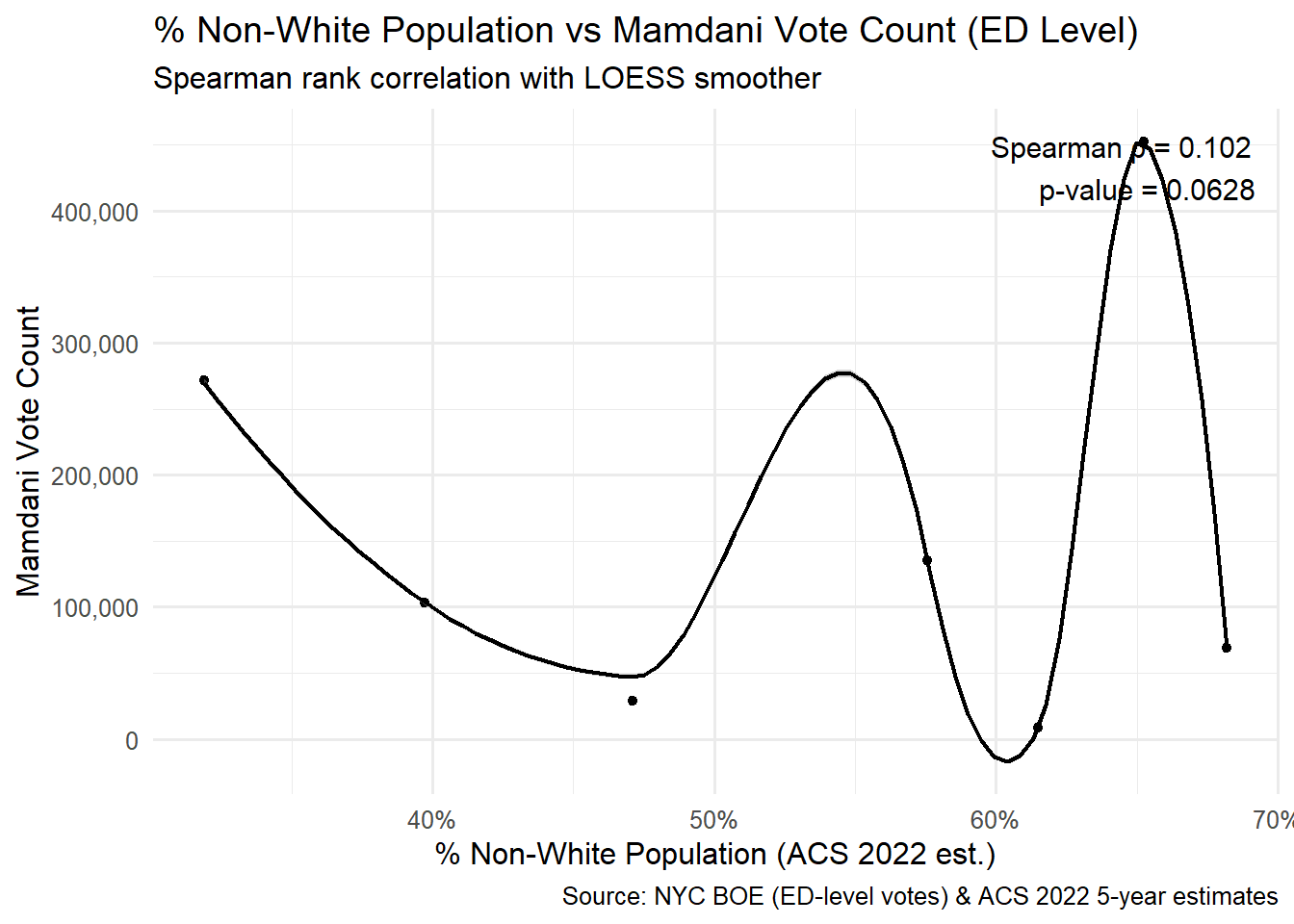
A spearman rank correlation graph showing the relationship between median household income and number of Mamdani votes
Discussion & Interpretation
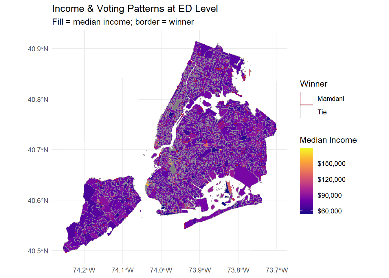
In the Income & Voting Patterns at ED Level map we see at an election district level median incomes. The data used is ACS 2023 data spatially joined and appropriated using logic that applies the majority income category to the prevailing polygon geography (election districts). We see overall there are pockets of higher median income ($150,000 and above) as well as pockets of lower income ($60,000 and below) zooming into the higher income pockets, they are concentrated in what is near downtown Brooklyn and the financial district in Manhattan.
The same logic was used to create the Race and Voting Patterns at ED level map. There is some overlap between median income and a lower proportion of non-White residents within the same geography when we compare the two maps. According to recent census bureau data white non-hispanics make up roughly 31% of New York City’s current population. This data is further expanded upon using spearman scatter plots. A LOESS smoother was added to show where relationships between the correlation (Mamdani votes x median income, Mamdani votes x non-white percentage) strengthen and weaken.
A Spearman rank correlation was used to assess the monotonic relationship between median household income and Mamdani vote counts at the election district level. Concerning median income, The correlation indicates a modest association, suggesting that districts with higher median incomes tend to contribute somewhat more Mamdani votes in absolute terms. However, the LOESS smoother reveals a nonlinear pattern, with vote accumulation concentrated in middle-income districts and diminishing marginal increases at the highest income levels. This suggests that Mamdani’s electoral support is geographically concentrated rather than uniformly stratified by income.
Concerning Race, The analysis indicates a positive monotonic association, suggesting that districts with higher percentages of non-white residents tend to contribute more Mamdani votes in absolute terms. The LOESS smoother reveals a nonlinear pattern, with vote accumulation increasing through middle-to-high non-white districts and flattening at the highest levels of racial concentration. This pattern suggests that Mamdani’s electoral support is geographically concentrated within non-white and racially mixed districts rather than uniformly increasing across the racial distribution.
It is helpful to have these spearman correlations as a limitation of this spatial allocation is that the small geographies of election districts do not capture larger trends of income distribution or racial distribution in the same way a larger geography might. In areas such as the Upper East Side where we know there is a high concentration of high income earners, the geography of the election districts capture more diversity.
When we look at the specific geographies noted in the introduction we do see an east west cline with relatively higher median income/low non-white residents near downtown Brooklyn (the commie corridor - west) towards Bushwick (the commie corridor - east) which has a lower median income and higher proportion of non-white residents. The financial district is interesting in that the most racially diverse, and relatively poorer election districts are the ones that voted for Mamdani. Looking at the South Bronx there are two districts that Mamdani won and they are of middling diveristy and income. Interestingly no election districts adjacent to central park on the Upper East Side are districts that Mamdani won. Perhaps the most interesting geography, that of Staten Island the only borough Cuomo won, shows that racially diverse election districts voted for Mamdani.
Conclusion
Mamdani ran a dynamic and successful campaign that spoke to issues affecting a broad swath of New Yorkers. In particular, he spoke to the issue of public safety and affordability whilst also keeping in step with issues of national origin, increasing violence towards immigrants, and took a strong stance against ICE. When we look at the data we see that this message rang through for New Yorkers who are middle to low income and New Yorkers who represent the increasing diveristy of the city.
I believe that this data shows that there is value in political candidates speaking to issues that their constiuants face and the campaign members, supporters, staffers, and Mamdani himself did a good job putting their finger on the pulse of the city. This data is an incomplete look at the people who have put their hopes into this new mayoral administration and I believe that a more thorough analysis looking at data on a borough level could be helpful for any efforts to identify these emergent political blocs.